Chapter Template | STEM Nexus

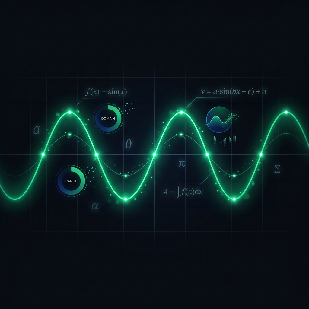
1. Introduction to Functions

At its core, a function is a relationship connecting one set of elements to another. Think of it as a machine: you provide an input, the machine processes it according to a specific rule, and it produces exactly one output.

"A function is a magical box that transforms the world, one value at a time. It demands predictability: one input, one unique output."

2. Key Terminology

To truly master functions, it's essential to understand the vocabulary used to describe them:

Domain: The set of all possible inputs (x-values).
Codomain & Range: The set of all possible outputs (y-values) that actually occur.
Mapping: The rule that pairs each element of the domain with an element in the range.

Interactive GeoGebra Plot

3. Types of Functions

Functions come in many flavours, each with distinct characteristics and graphical shapes. Understanding these types is crucial for recognising patterns in data and choosing the right model for a given situation.

Four types of mathematical functions: linear, quadratic, exponential, and hyperbolic

The Four Core Function Families Linear · Quadratic · Exponential · Hyperbolic — each with a unique graphical signature

Graph Theory

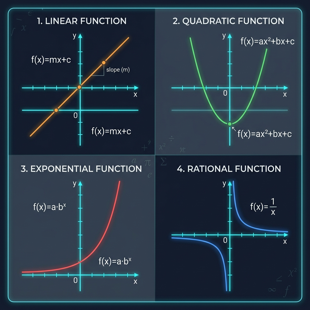
3.1 Linear Functions

A linear function has the general form $ f(x) = mx + c $, where m is the gradient (slope) and c is the y-intercept. The graph is always a straight line. Linear functions model constant rates of change — for example, a car travelling at a steady speed of 60 km/h.

$$ f(x) = mx + c $$

3.2 Quadratic Functions

Quadratic functions take the form $ f(x) = ax^2 + bx + c $. Their graphs are parabolas — U-shaped curves that open upward when $ a > 0 $ and downward when $ a < 0 $. The turning point (vertex) represents either a maximum or minimum value.

$$ f(x) = ax^2 + bx + c $$

3.3 Exponential Functions

Exponential functions have the form $ f(x) = a \cdot b^x $. When $ b > 1 $, the function models exponential growth (population growth, compound interest). When $ 0 < b < 1 $, it models exponential decay (radioactive decay, depreciation). The key feature is that the rate of change is proportional to the current value.

"The greatest shortcoming of the human race is our inability to understand the exponential function." — Albert A. Bartlett

3.4 Hyperbolic Functions

The basic hyperbola $ f(x) = \frac{a}{x} + q $ has two branches that approach but never touch the axes (asymptotes). These functions are useful for modelling inversely proportional relationships — for example, pressure and volume of a gas at constant temperature (Boyle's Law).

4. Evaluating Functions

When evaluating a function, you substitute a specific value into the equation. For example, if $ f(x) = 2x + 3 $, then evaluating the function at $ x = 4 $ gives $ f(4) = 2(4) + 3 = 11 $.

Evaluation extends beyond simple substitution. You can evaluate functions at expressions, other functions, or even complex numbers:

$ f(a + h) $: Substitute the entire expression $ (a + h) $ for every occurrence of $ x $.
$ f(-x) $: Replace every $ x $ with $ -x $. This is the foundation for testing symmetry (even/odd functions).
$ f(g(x)) $: First evaluate the inner function $ g(x) $, then use that result as the input for $ f $.

5. Transformations of Functions

One of the most powerful ideas in mathematics is that you don't need to memorise every possible graph. Instead, you can start from a parent function and apply transformations to obtain any related graph.

5.1 Vertical & Horizontal Shifts

Adding a constant q to a function shifts its graph vertically: $ f(x) + q $ moves the graph up by q units (or down if q is negative). Similarly, $ f(x - p) $ shifts the graph right by p units.

5.2 Reflections

Multiplying by $ -1 $ creates reflections. $ -f(x) $ reflects the graph in the x-axis (flipping it upside down), while $ f(-x) $ reflects it in the y-axis (creating a mirror image).

5.3 Stretches & Compressions

The parameter a in $ a \cdot f(x) $ controls a vertical stretch (if $ |a| > 1 $) or compression (if $ 0 < |a| < 1 $). Similarly, $ f(bx) $ applies a horizontal compression when $ |b|> 1 $ and a horizontal stretch when $ 0 < |b| < 1 $.

"Mathematics is not about numbers, equations, computations, or algorithms: it is about understanding." — William Paul Thurston

Visual demonstration of vertical and horizontal shifts, reflections, and stretches on function graphs

Visual Reference

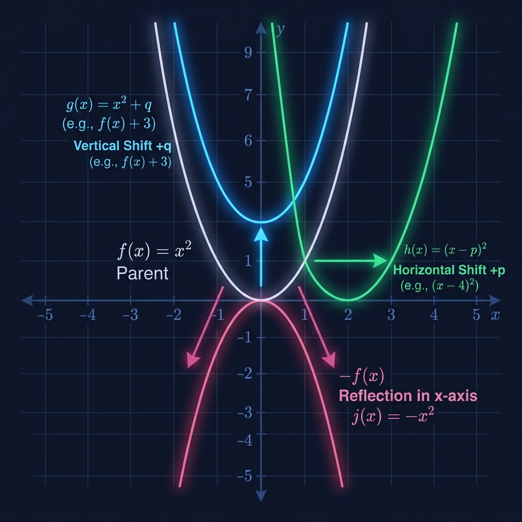
Transformations at a Glance

Every transformation modifies the parent function in a predictable, systematic way — mastering these patterns means you can sketch any related graph without computing new points.

Vertical shift: $ f(x) + q $ — slides the graph up or down.

Horizontal shift: $ f(x - p) $ — moves the graph left or right.

Reflection: $ -f(x) $ — flips the graph across the x-axis.

Stretch / Compress: $ a \cdot f(x) $ — scales the graph vertically.

6. Composition of Functions

Function composition combines two functions by using the output of one as the input of another. Written as $ (f \circ g)(x) = f(g(x)) $, you first evaluate the inner function $ g(x) $, then feed its result into $ f $.

Composition is not commutative — in general, $ f(g(x)) \neq g(f(x)) $. This is an important distinction that catches many students off guard.

$$ (f \circ g)(x) = f(g(x)) $$

Worked Example: Let $ f(x) = 2x + 1 $ and $ g(x) = x^2 $.

$ f(g(x)) = f(x^2) = 2(x^2) + 1 = 2x^2 + 1 $
$ g(f(x)) = g(2x + 1) = (2x + 1)^2 = 4x^2 + 4x + 1 $

Notice how the two compositions yield entirely different results!

7. Inverse Functions

An inverse function "undoes" the operation of the original function. If $ f(a) = b $, then $ f^{-1}(b) = a $. Graphically, the inverse is a reflection of the original function across the line $ y = x $.

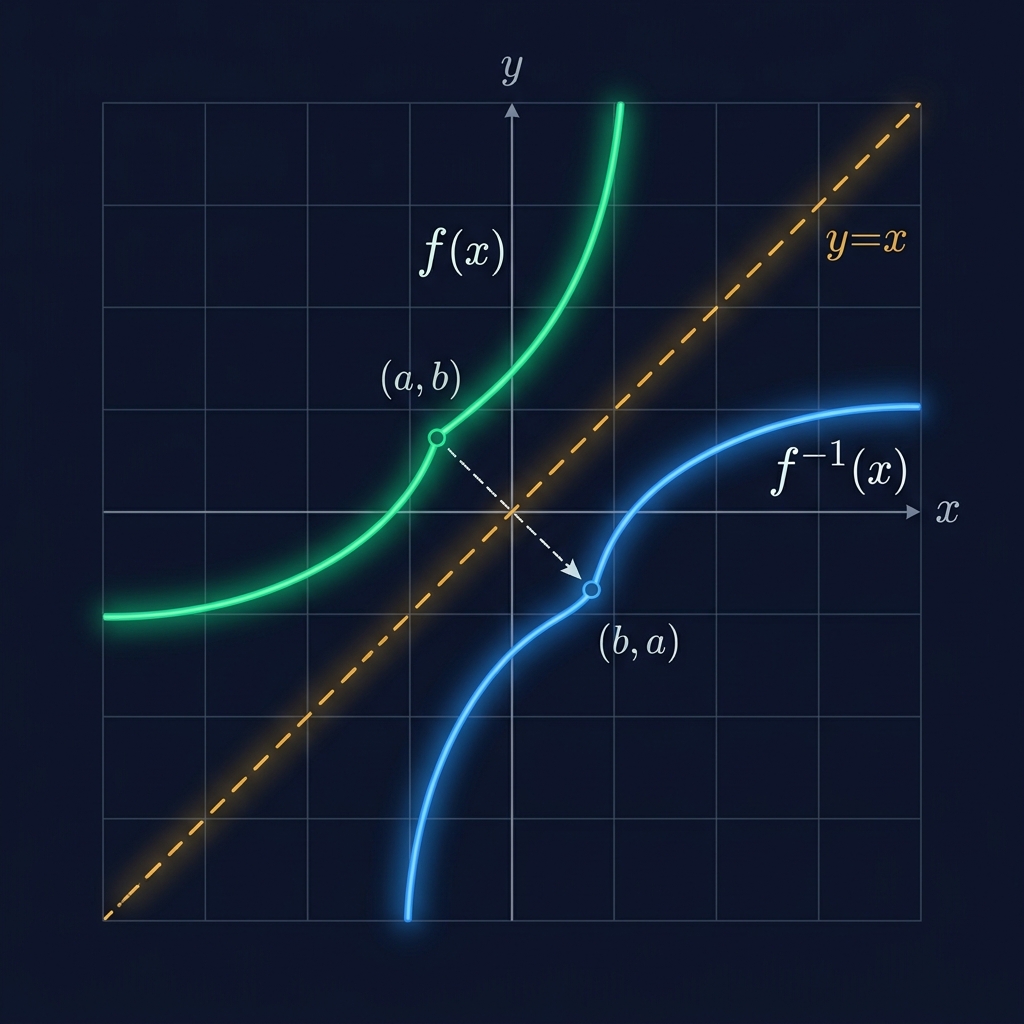
Inverse function diagram showing f(x) and f-inverse(x) as mirror images across the line y = x

Key Insight

The Mirror Principle

The graph of $ f^{-1}(x) $ is the mirror image of $ f(x) $ reflected across the line $ y = x $. This symmetry is the visual fingerprint of every inverse relationship.

Not every function has an inverse. A function must be one-to-one (injective) — meaning each output maps to exactly one input. Use the Horizontal Line Test: if any horizontal line crosses the graph more than once, no inverse exists without restricting the domain.

Finding an Inverse

To find the inverse of a function algebraically:

Step 1: Replace $ f(x) $ with $ y $.
Step 2: Swap $ x $ and $ y $.
Step 3: Solve the new equation for $ y $.
Step 4: Write the result as $ f^{-1}(x) $.

$$ f(f^{-1}(x)) = f^{-1}(f(x)) = x $$

8. Real-World Applications

Science and mathematics applications: physics, finance, and biology

Functions aren't just abstract mathematical objects — they are the backbone of modelling the real world. Almost every measurable relationship in science, engineering, economics, and daily life can be described using functions.

8.1 In Physics

The motion of a projectile follows a quadratic function: $ h(t) = -\frac{1}{2}gt^2 + v_0t + h_0 $, where $ g $ is gravitational acceleration, $ v_0 $ is initial velocity, and $ h_0 $ is initial height. Understanding this function allows engineers to design everything from bridges to spacecraft trajectories.

Kinematics Explorer (Displacement)

Adjust initial velocity $ v_0 $, time $ t $, and acceleration $ a $ to see the resulting displacement $ s $:

$ v_i $ (m/s): 0 $ t $ (s): 4 $ a $ (m/s²): 1.2

8.2 In Finance

Compound interest is modelled by an exponential function: $ A = P\left(1 + \frac{r}{n}\right)^{nt} $. Banks, investors, and financial planners depend on this function daily. Understanding its behaviour helps make informed decisions about loans, savings, and investments.

Annuity Future Value Explorer

See how monthly contributions grow over time. Modify Monthly Payment (PMT), Interest Rate (r), and Years (n).

PMT ($/mo): 200 Rate (r): 6.0% Years (n): 20

8.3 In Biology

Population growth often follows logistic functions, which start with exponential growth but eventually level off due to limiting factors like food, space, and competition. The logistic model $ P(t) = \frac{K}{1 + Ce^{-rt}} $ captures this behaviour elegantly, where $ K $ is the carrying capacity of the environment.

"The book of nature is written in the language of mathematics." — Galileo Galilei

9. Chapter Summary

In this chapter, we explored the foundational building blocks of mathematical functions. Let's recap the key takeaways:

Definition: A function maps each input to exactly one output.
Terminology: Domain, codomain, range, and mapping are essential vocabulary.
Types: Linear, quadratic, exponential, and hyperbolic functions each have unique characteristics.
Evaluation: Substitution is the core technique for finding function values.
Transformations: Shifts, reflections, and stretches modify parent functions systematically.
Composition: Chaining functions together creates new, more complex functions.
Inverses: Inverse functions reverse the mapping of the original function.
Applications: Functions model real-world phenomena across every scientific discipline.

With these tools, you are now equipped to analyse, graph, and interpret a wide variety of functional relationships. In the next chapter, we will put these concepts to work in the context of Financial Mathematics.